Last time we saw how Polynomial regression can fit complex patterns, but as we increased the degree of the polynomial, we encountered overfitting; the model performs well on the training data but poorly on unseen test data.
Regularization helps combat overfitting by adding a penalty term to the loss function, discouraging overly complex models. We’ll explore three common regularization techniques: Ridge, Lasso, and Elastic Net.
Ridge Regression
Ridge adds a penalty proportional to the squared magnitude of coefficients:
$$ \text{Loss} = \text{MSE} + \alpha \sum_j w_j^2 $$
- Encourages smaller coefficients
- Doesn’t eliminate features completely
- Tends to reduce model complexity and variance
Lasso Regression
Lasso adds a penalty proportional to the absolute value of coefficients:
$$\text{Loss} = \text{MSE} + \alpha \sum_j |w_j|$$
- Can shrink some coefficients to exactly zero
- Useful for feature selection
- Produces sparse models
import numpy as np
from sklearn.pipeline import make_pipeline
from sklearn.model_selection import train_test_split
from sklearn.preprocessing import PolynomialFeatures, StandardScaler
from sklearn.linear_model import Lasso, Ridge, ElasticNet

X = np.random.rand(100)
y = 5*np.sin(3 * np.pi * X) + np.random.normal(0, 2, X.shape)

X_train, X_test, y_train, y_test = train_test_split(X, y, test_size=0.5, random_state=42)

degree = 40

model = make_pipeline(PolynomialFeatures(degree), StandardScaler(), LinearRegression())
model.fit(X_train, y_train)

lasso_model = make_pipeline(PolynomialFeatures(degree), StandardScaler(), Lasso(0.1,max_iter=10000))
lasso_model.fit(X_train, y_train)

ridge_model = make_pipeline(PolynomialFeatures(degree),StandardScaler(), Ridge(0.0001))
ridge_model.fit(X_train, y_train)
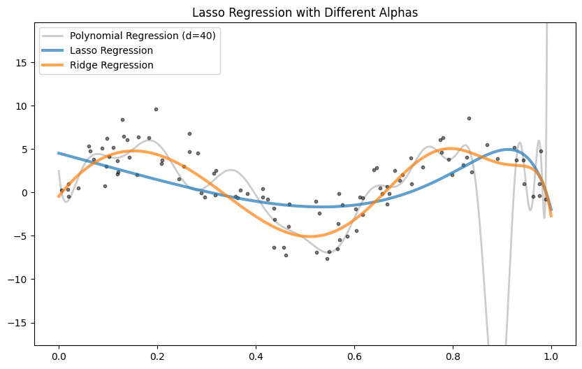
In this example Ridge Regression works best, since the sinus function is non polynomial.
n_samples = 100
X = np.random.uniform(-5, 5, size=(n_samples, 1))
y_true = 0.3 * X[:,0] * X[:,0] * X[:,0]
y = y_true + np.random.normal(scale=6.0, size=n_samples)

X_train, X_test, y_train, y_test = train_test_split(X, y, test_size=0.5, random_state=42)

degree = 40

model = make_pipeline(PolynomialFeatures(degree), StandardScaler(), LinearRegression())
model.fit(X_train, y_train)

lasso_model = make_pipeline(PolynomialFeatures(degree), StandardScaler(), Lasso())
lasso_model.fit(X_train, y_train)

ridge_model = make_pipeline(PolynomialFeatures(degree),StandardScaler(), Ridge())
ridge_model.fit(X_train, y_train)
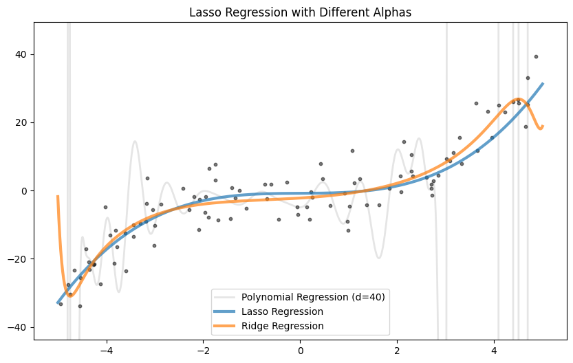
In the case of this function lasso regularization works best, as it selects the relevent features.
So Ridge prevents coefficients from exploding, but keeps all of them. Usefull when you suspect many features to be useful (dense solution). Or when features are highly correlated.
Lasso performs feature selection by setting some coefficients to zero But it can behave erratically when features are highly correlated — arbitrarily picking one and ignoring the others.
Elastic Net
Elastic Net combines Ridge and Lasso, giving you the stability of Ridge and the sparsity of Lasso.
$$ \text{Loss} = \text{RSS} + \alpha \cdot \left[ \rho \cdot \sum |w_i| + (1 - \rho) \cdot \sum w_i^2 \right] $$
- $\alpha$: overall regularization strength.
- $\rho$ (or
l1_ratioin scikit-learn): mix between Lasso ($\ell_1$) and Ridge ($\ell_2$).
It is usefull, when you have many correlated features, but you want sparsity.
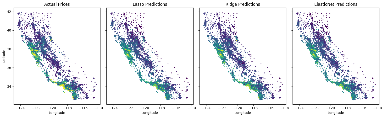
Here is an example using real data, comparing the 3 approaches:
from sklearn.datasets import fetch_california_housing
from sklearn.linear_model import LassoCV, RidgeCV, ElasticNetCV

data = fetch_california_housing()
X, y = data.data, data.target
longitude = X[:, data.feature_names.index('Longitude')]
latitude = X[:, data.feature_names.index('Latitude')]

degree = 5
lasso = make_pipeline(PolynomialFeatures(degree), StandardScaler(), LassoCV(n_jobs=8))
ridge = make_pipeline(PolynomialFeatures(degree), StandardScaler(), RidgeCV())
elastic = make_pipeline(PolynomialFeatures(degree), StandardScaler(), ElasticNetCV(n_jobs=8)

lasso.fit(X, y)
ridge.fit(X, y)
elastic.fit(X, y)
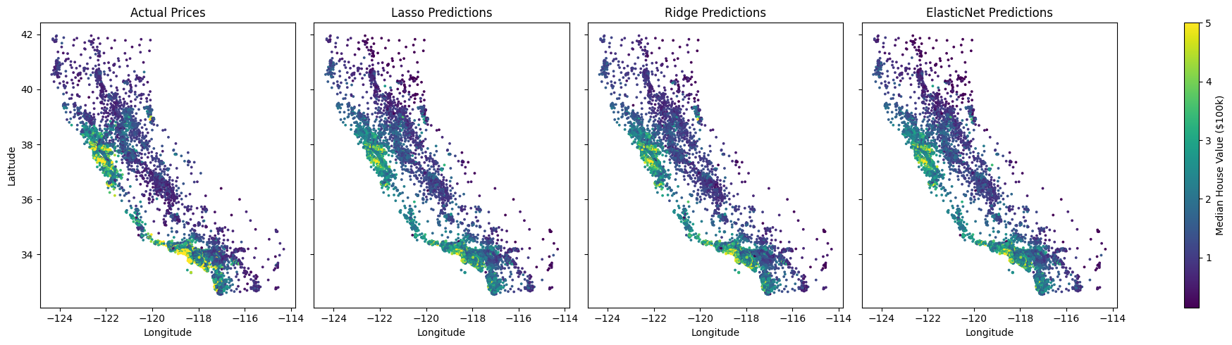
Lasso MSE: 0.4795
Ridge MSE: 0.3778
ElasticNet MSE: 0.4766