
Yesterday, we explored how to train a binary classifier using logistic regression. Today, we’ll generalize that idea to handle multiple classes. This generalization is known as softmax regression, or multinomial logistic regression.
The Idea
In binary logistic regression, we used a single score function to compute the probability of a class. For multiclass classification, we extend this by defining one score function per class:
$$ s_k(x) = \theta_k^T x $$
Here, $s_k(x)$ is the score for class $k$, and $\theta_k$ is the parameter vector for that class.
To turn these scores into probabilities that sum to one, we apply the softmax function:
$$ \hat{p}_k = \sigma (x)_k = \frac{\exp(s_k(x))}{\sum^{K}_j \exp(s_j(x))} $$
This gives us a vector of probabilities over all $K$ classes. The predicted class is simply the one with the highest probability:
$$ \hat{y} = \arg\max_k ~ \sigma(x)_k $$
Training with Cross-Entropy Loss
To train the model, we use the cross-entropy loss, which compares the predicted probability distribution with the true distribution (a one-hot vector for classification):
$$ J(\Theta) = -\frac{1}{m} \sum_{i=1}^m \sum_{k=1}^K y^{(i)}_k \log(\hat{p}^{(i)}_k) $$
Here, $y^{(i)}_k$ is 1 if class $k$ is the true class for example $i$, and 0 otherwise.
Softmax in Action: Iris Dataset
Let’s see how softmax classification performs on the classic Iris dataset, using the same features we used for logistic regression: petal length and petal width.
from sklearn import datasets
from sklearn.linear_model import LogisticRegression

iris = datasets.load_iris()
X = iris["data"][:, [2,3]]
y = iris["target"]

softmax = LogisticRegression()
softmax.fit(X, y)
import matplotlib.pyplot as plt
import numpy as np
from matplotlib.colors import ListedColormap

k=3
# Meshgrid
x_min, x_max = X[:, 0].min() - 2, X[:, 0].max() + 2
y_min, y_max = X[:, 1].min() - 2, X[:, 1].max() + 2
xx, yy = np.meshgrid(np.linspace(x_min, x_max, 300),
                     np.linspace(y_min, y_max, 300))
grid = np.c_[xx.ravel(), yy.ravel()]

# Softmax probabilities: shape (n_points, n_classes)
probs = softmax.predict_proba(grid)
probs = probs.reshape(xx.shape[0], xx.shape[1], -1)  # reshape to grid shape

# Predicted class at each grid point
predicted_class = np.argmax(probs, axis=2)

# Plotting
plt.figure(figsize=(10, 5))

labels = iris.target_names

cmap = plt.get_cmap("Spectral")
cmap = cmap(np.linspace(0.2, 0.8, 256))
cmap = ListedColormap(cmap)

plt.contourf(xx, yy, predicted_class, cmap=cmap, levels=20, alpha=0.7)

plt.contour(xx, yy, predicted_class, levels=np.arange(probs.shape[2] + 1) - 0.5, colors='black', linestyles=':', linewidths=2, alpha=0.7)
for i in range(k):
    plt.scatter(X[y==i][:, 0], X[y == i][:, 1], color=cmap(i/2), label=labels[i], edgecolor='k', alpha=1, s=50)

# Draw decision boundaries (contours between classes)

# Labels and legend
plt.xlabel("Petal length (cm)")
plt.ylabel("Petal width (cm)")
plt.title("Softmax Classification of Iris Dataset")
plt.legend(loc="upper left")
plt.tight_layout()
plt.show()
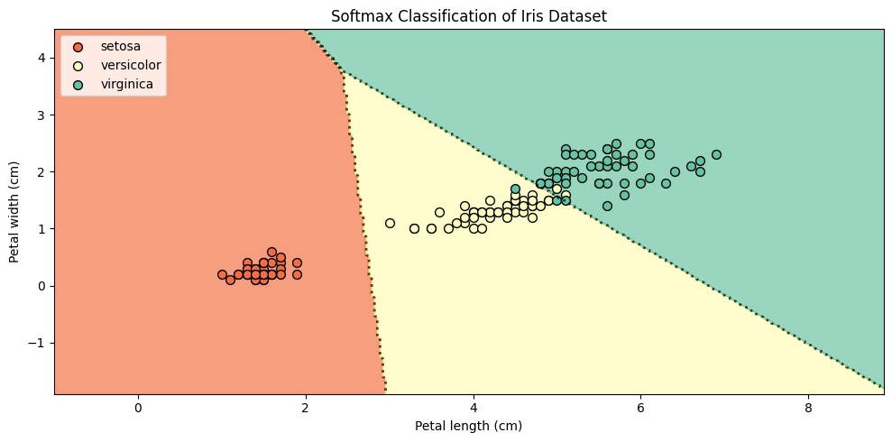
This visualization shows how softmax regression partitions the feature space into decision regions for each class. Unlike binary logistic regression, softmax handles all classes in one unified model.